Texts Are More than Notes, They Are Data: A Glimpse into How Machines Understand Text

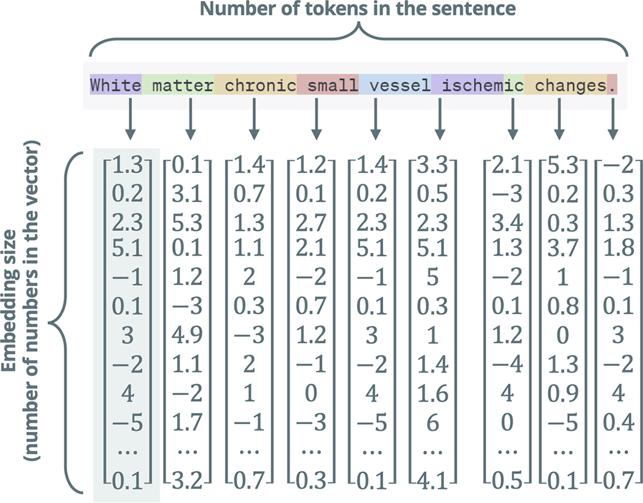
Figure 1: The input of the transformer model is a set of vectors comprising a vector for each token. Different background colors in the sentence, “White matter chronic small vessel ischemic changes” show each token. The size of each vector is the number of numbers in it, referred to as embedding size. These numbers encode a different meaning for each word.

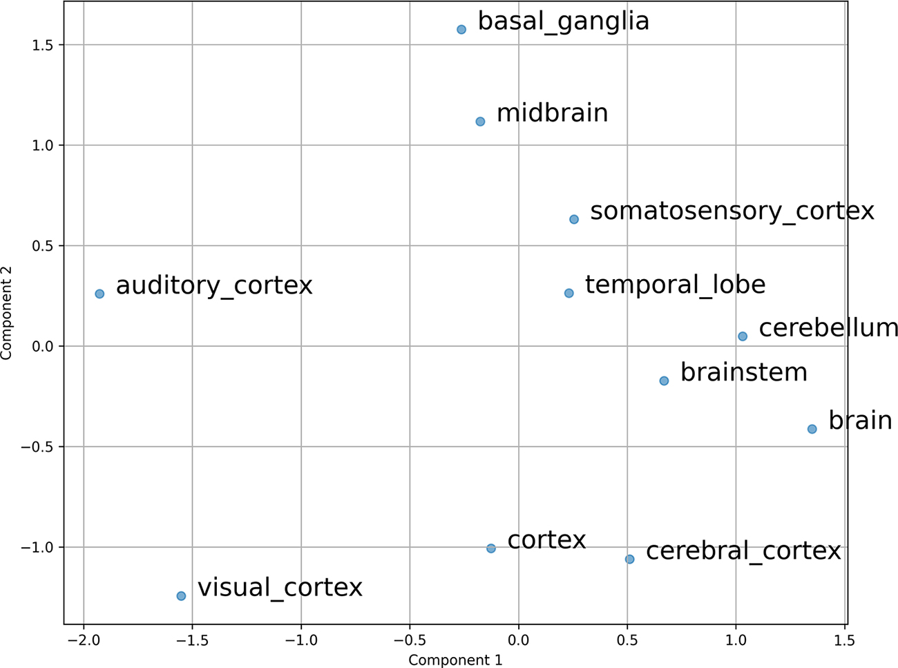
Figure 2: Graph shows an example of the closest words to the word brainstem in Google’s Word2Vec embedding space. This example shows the closest words to brainstem are cerebellum, brain , and temporal_lobe . One of the farthest words to brainstem is visual_cortex . Principal component analysis was used to reduce the embedding size to two arbitrary dimensions so it can be better viewed on a two-dimensional plane. The components (components 1 and 2) are the two principal components and carry no meaningful information for humans.

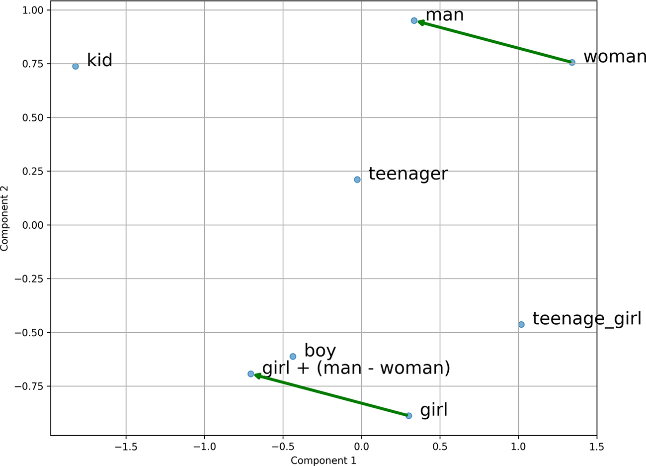
Figure 3: Graph shows an example of the relationship between words in Google’s Word2Vec embedding space. Principal component analysis was used to reduce the embedding size to two dimensions so it can be better viewed on a two-dimensional plane. Note that despite the fact that the words woman, man, boy , and girl reside in different areas of the vector space, the distance between the words man and woman is similar to the distance between the words boy and girl . Mathematically, subtracting the vector for woman from that of man and adding the result to girl yields a point in the embedding space that lies near boy . The similar distance means that the embedding space encodes the analogy that boy is to girl as man is to woman.

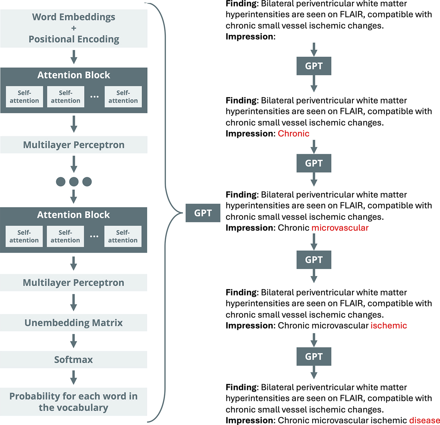
Figure 4: The overall structure of a generative pretrained transformer (GPT) model. After positional encoding is applied to the word embeddings, a series of attention blocks and multilayer perceptrons are applied to the embeddings. Ultimately, an unembedding matrix generates scores for each word in the vocabulary. These scores are transformed into probabilities by the softmax function. Then, the next word in the sentence is chosen by sampling it from the generated probability distribution. That process is repeated until the model predicts the end-of-sequence token. FLAIR = fluid-attenuated inversion recovery.

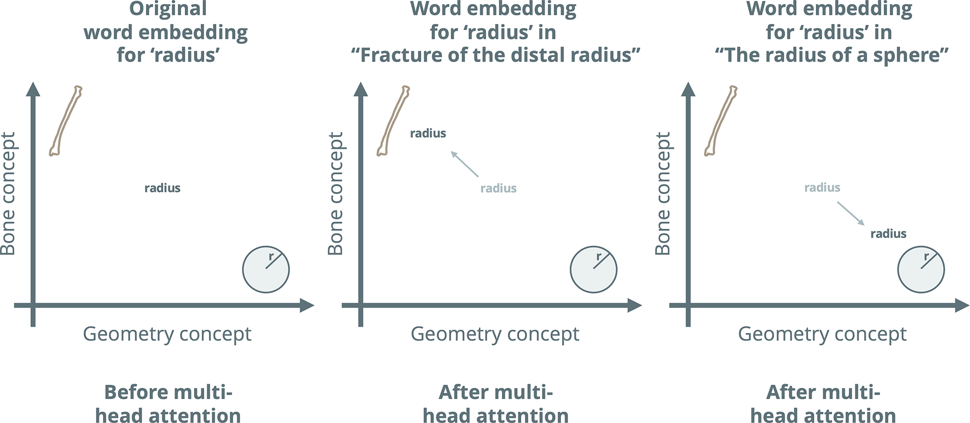
Figure 5: Graphs show how transformers self-adjust word embeddings based on other words in a sentence using a self-attention mechanism. On the left side of the figure, the original embedding of the word radius lies between its two possible meanings (bone or geometric). In the middle of the figure, after passing through an attention block, the embedding for the word radius lies closer to the bone radius if the sentence is “Fracture of the distal radius.” On the right part of the figure, after passing through an attention block, the embedding for the word radius lies closer to the geometric radius if the sentence is “The radius of a sphere.” r = radius of a circle.

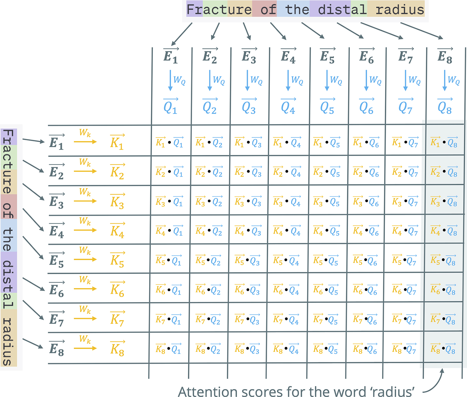
Figure 6: Image shows self-attention in a transformer, part 1 (queries and keys). Think of each word in the sentence as a colleague in a meeting: Each colleague can ask questions (queries) and offer information (keys). The query vectors capture what each word is seeking in the other words, whereas the key vectors capture what each word has to offer. By taking the dot product between queries and keys, the model measures how closely two words are related; a larger value means they have more in common. A softmax function then turns these raw scores into probabilities that show how strongly each word is influenced by every other word. For example, when radius looks at fracture and distal in the sentence, “Fracture of the distal radius,” it might assign higher probabilities to these words because fracture indicates an injury relevant to a bone and distal specifies an anatomic location relevant to the radius. The query vector is Q i = W q E j . The key vector is K i = W k E j . W q , W k are learned projection matrices for queries and keys, respectively; and subscripts from 1 through 8 denote word (or token) positions in the sentence. Attention scores are computed with dot products K i t · Q i , where subscripts i and j indicate word (or token) posititions in the sentence. E i = embedding of the i-th word.

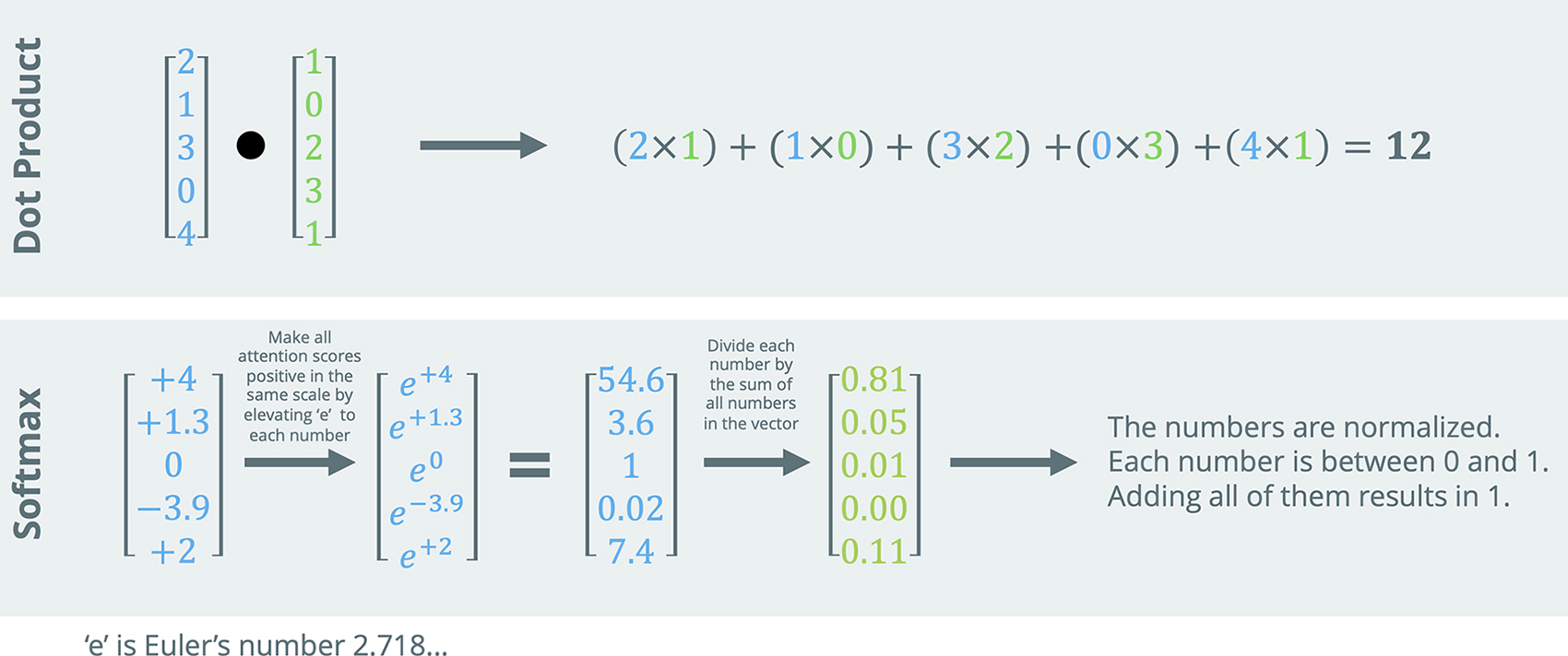
Figure 7: Image shows dot product and softmax in transformer self-attention mechanisms. The dot product is a way to quantify the relationship between two words by multiplying each component of their vectors and then summing them up. A positive result means they are correlated in some sense, and a higher positive result means they share more context. The softmax function then converts these results into probabilities that add up to 1, which makes it easier to see which word has the highest influence. In the same sentence, if the dot product between fracture and radius is much larger than the dot product of filler words like of or the , the softmax will emphasize the word fracture as a key influencer of radius .

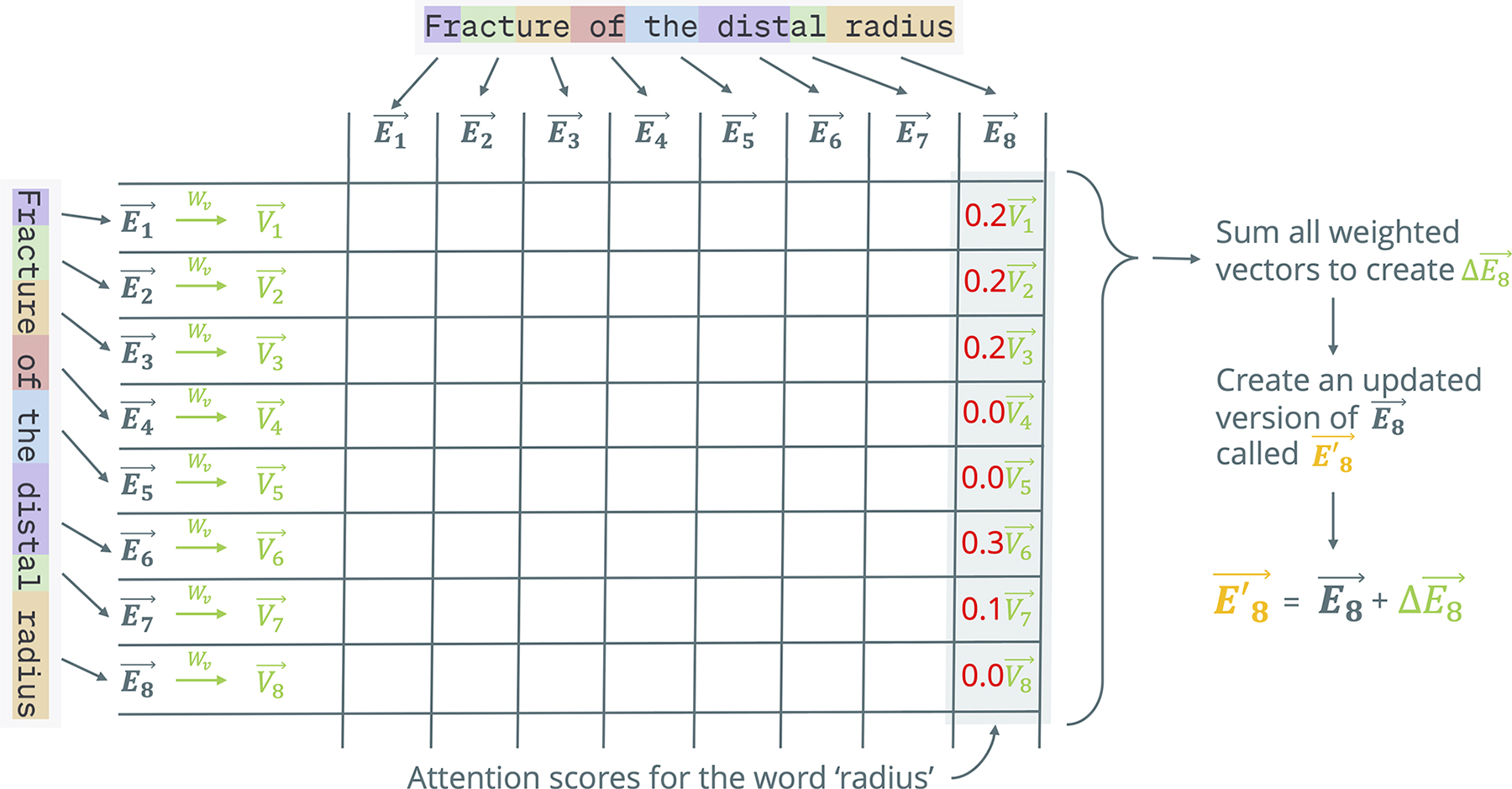
Figure 8: Graph shows self-attention in a transformer, part 2 (values). After determining which words matter to one another using the keys and queries, the model collects the actual “content” that each word can contribute by multiplying the original word embeddings by a value matrix. The probabilities from Figure 6 are then used to create a weighted sum of these value vectors, producing a difference vector (ΔE) that is added to the original embedding. This means that the concept of radius is updated by whatever the words fracture and distal contribute. For instance, fracture contributes to the idea of bone injury, and distal contributes to the idea of an anatomic location. By adding these influences, the updated embedding for radius captures the meaning of “a forearm bone with a fracture specifically at its distal region,” which is a crucial context shift for radiologic interpretation. Value vector is V i = W v E i . Attention weights (in red, from Figure 6 ) indicate the contribution of each V i to update E 8 (for radius). Updated embedding is E’ 8 = E 8 + Δ E 8 . Subscripts from 1 through 8 index word positions in the sentence. E i = embedding of the i-th word, W v = learned projection matrix for values, Δ E 8 = weighted sum of values.

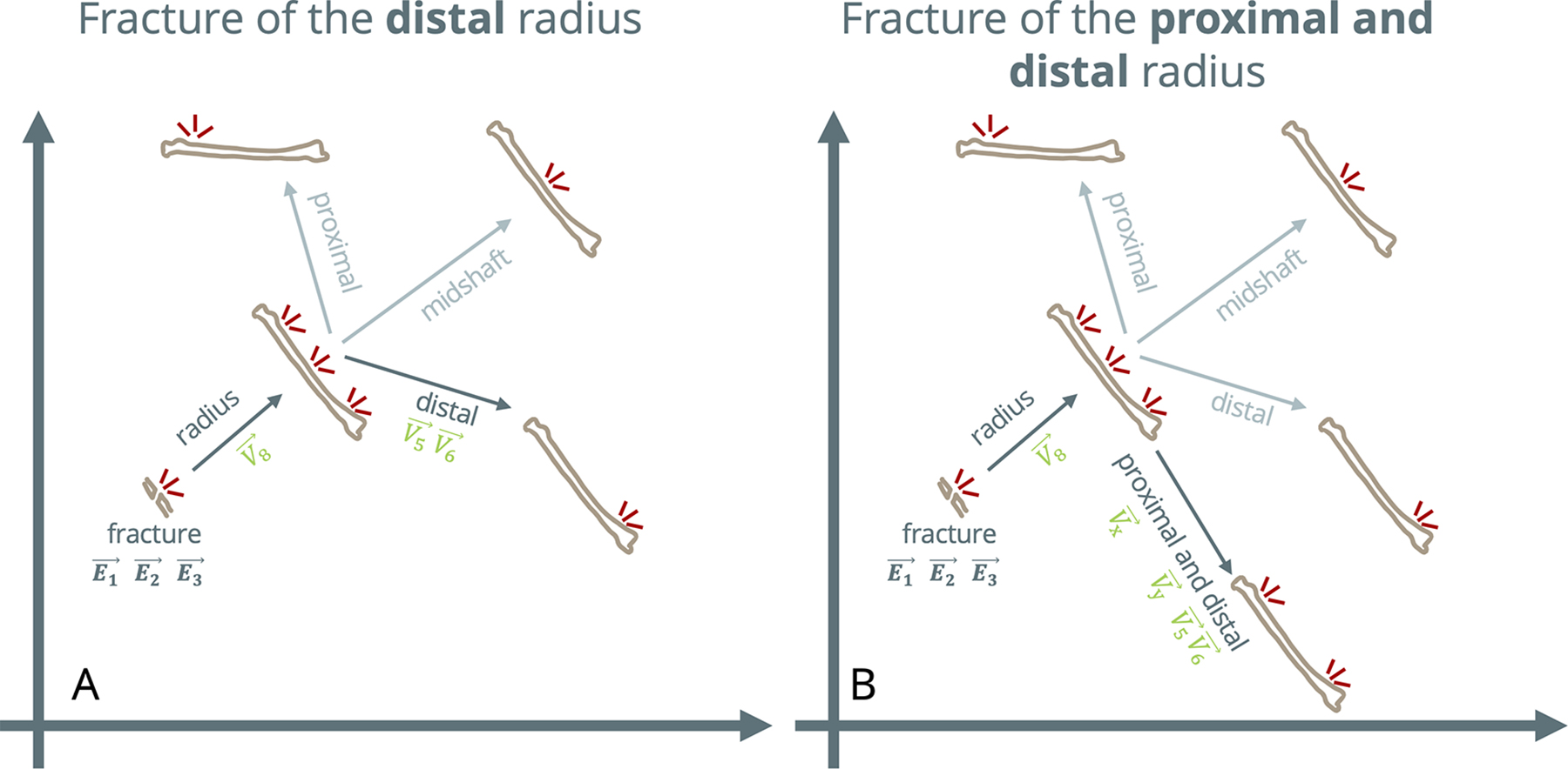
Figure 9: Plots show a simplified explanation of how the word embedding is changed by the Values of the surrounding words in a transformer. (A) The sentence, “Fracture of the distal radius” is used as an example. The original embedding for fracture (E 1 , E 2 , E 3 ) has a general meaning (broken bone). After applying the Value vector V 8 for the word radius , the embedding for fracture now means a fracture of the radius. Then, applying the Value vectors for distal (V 5 , V 6 ), the embedding for fracture encodes a more specific meaning of fracture in the distal radius. Note that if the sentence had the words proximal or midshaft instead of distal , the final embedding would have ended in a different location in the embedding vector space. (B) The sentence, “Fracture of the proximal and distal radius” is used as an example. The original embedding for fracture (E 1 , E 2 , E 3 ) has a general meaning (broken bone). After applying the Value vector V 8 for the word radius , the embedding for fracture now means a fracture of the radius fracture. Then, applying the Value vectors for proximal and distal (V x , V y , V 5 , V 6 ), the embedding for fracture encodes a more specific meaning of fractures in the proximal and distal radius.

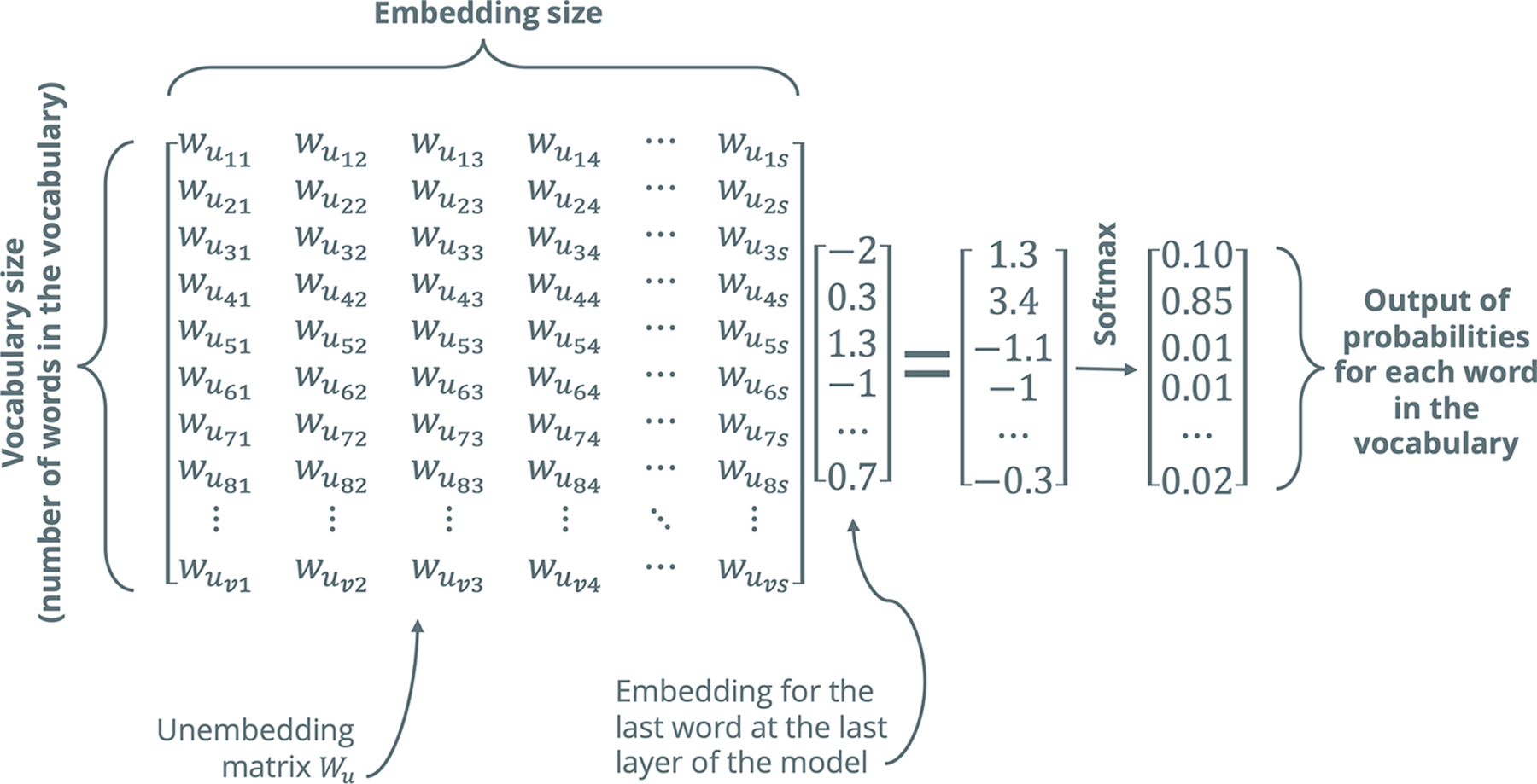
Figure 10: The last word embedding in the last layer of the transformer model is used to generate a vector containing probabilities for each word in the vocabulary, which is done by multiplying an unembedding matrix (W u ) by the last embedding. The output is a vector of scores for each word in the vocabulary, which is converted by softmax to a vector of probabilities. This vector is the reference to sample the next word for the input sentence. For example, if the partial impression reads “Impression: The findings suggest pneumonia, and we recommend further ___,” the model might predict evaluation , yielding “Impression: The findings suggest pneumonia, and we recommend further evaluation.”

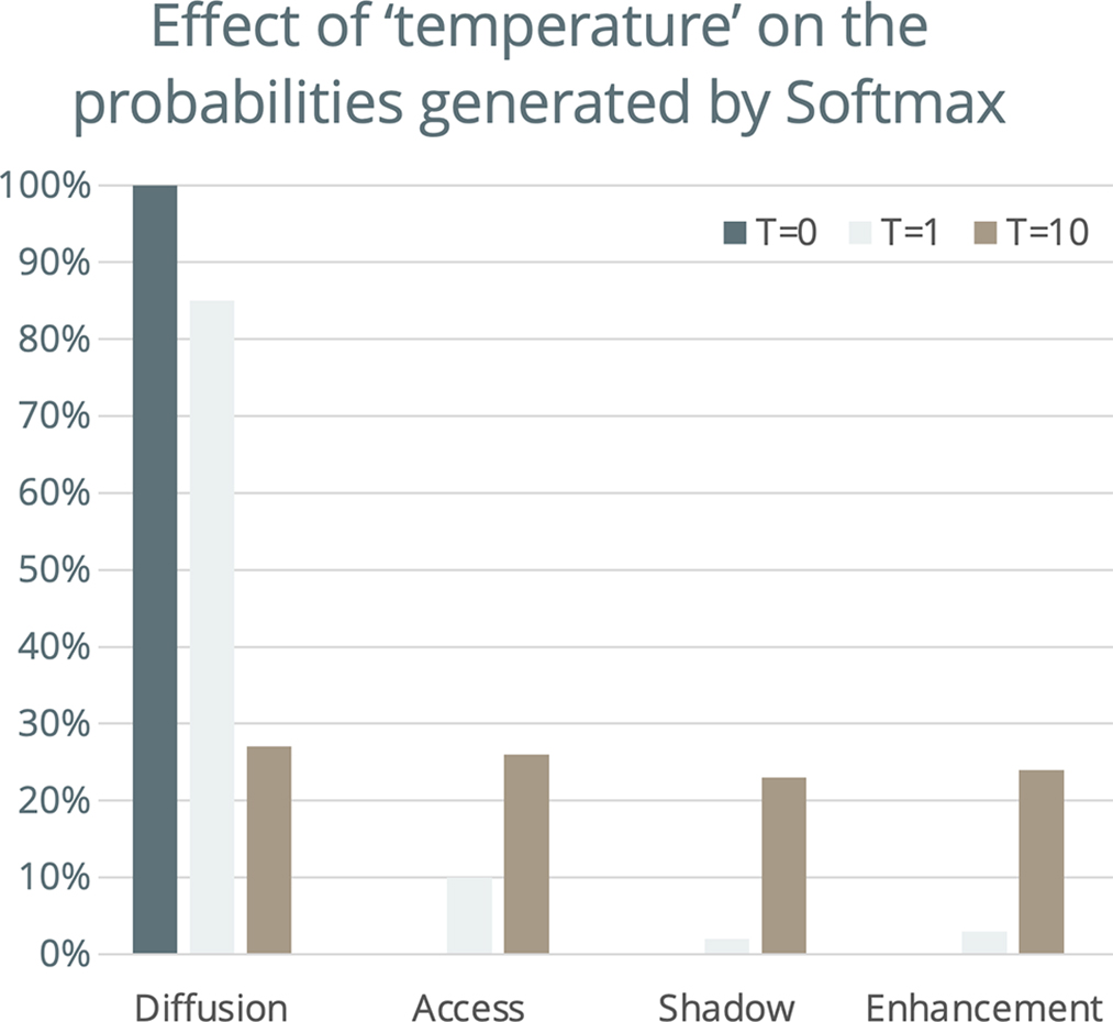
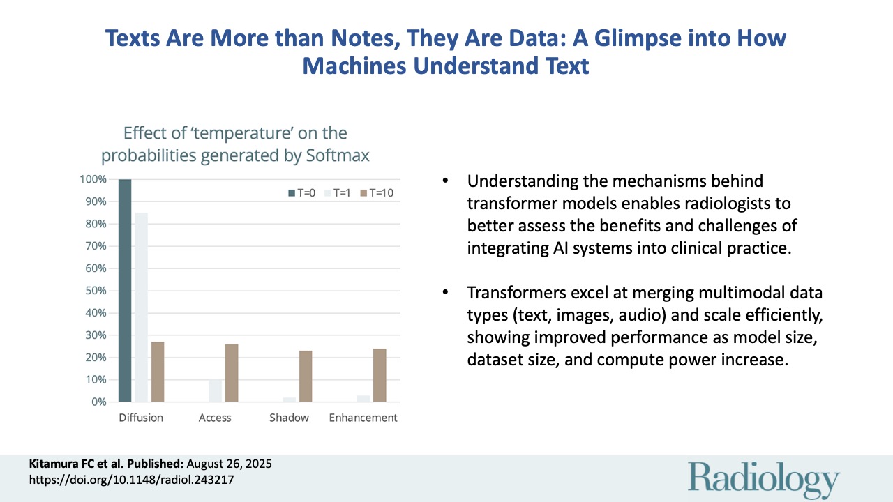
Figure 11: Graph shows how to adjust the softmax function to make the distribution of probabilities of the next word more or less pronounced by using temperature (T). T = 0 makes the most likely word to be chosen every time. T = 1 is the standard softmax function, whereas T > 1 starts to equalize the probabilities of all words, making the model produce more random output. Although temperature 0 makes the word diffusion the only possible option for the next word, with a temperature of 10 there is a similar chance that the words diffusion, access, shadow , or enhancement will be the next word. With T = 0, the only possible output is “Enhancing lesion with restricted diffusion.” With T = 10, it would be more likely that the output would be “Enhancing lesion with restricted access,” “Enhancing lesion with restricted shadow,” or “Enhancing lesion with restricted enhancement.” Hence, it is clear why high temperatures generate nonsensical outputs.

Figure 12: Image shows the challenges in using large language models (LLMs) in health care. The infographic depicts the significant challenges of using LLMs (eg, hallucination or confabulation, biases, privacy concerns, and automation bias).